


Policies that suppress or control COVID-19 prevent illness and save lives, but exact an economic toll. How should we balance lives and livelihoods to determine which policy is best? Richard Bradley, Alex Voorhoeve et al. compare benefit-cost and social welfare approaches to the pandemic.
Part 1: How can we measure the value of a life?
What is benefit-cost analysis?
Benefit-cost analysis evaluates a policy in terms of the sum of the monetary equivalents of its outcome. The most widely used monetary measure of the value of saving lives is the Value of a Statistical Life (VSL). This is derived from the rate at which people are willing to trade off small changes in their income against small changes in their risk of death. For example, suppose someone would accept a pay cut of $10,000 per year, but no more, to reduce their annual risk of mortality by 0.1%. Then the monetary value of their statistical life is $10,000/0.001 = $10,000,000. (What this means is that, if we had a population of 1,000 such people, then, in the aggregate, they would be willing to pay their fair share of $10,000,000 to reduce their individual risks of death by 0.1%, thereby lowering the expected number of deaths in their population by 1.)
The value of a statistical life derived from an individual’s preferences will depend on their income and wealth, which can have unacceptable consequences for benefit-cost analysis. In particular, the fact that someone who is well-off is likely to place a higher monetary value on risk reduction than someone who is less well-off implies that the interests of the well-off will count for more. By using a single value of a statistical life, such as the population average, this problem is avoided.
A new one arises, however, because such an average assigns the same value to every person’s life saved, independently of their age. But death is generally a more serious loss when it occurs earlier in life. Reasoning in terms of life years preserved rather than lives saved is therefore more sensible. This can be done by using the Value of a Statistical Life Year (VSLY) measure. This is obtained by dividing the average value of a statistical life of the population by the average life expectancy remaining. The value of saving the life of someone in any particular age cohort is then given by the product of the value of a statistical life year and the life expectancy remaining for the cohort.
Naturally, estimates of the value of statistical lives and life years will depend on a country’s income per capita. But they also vary considerably between different agents, even for a single country. For example, in the USA, the typical value of a statistical life used by government agencies is around $10,000,000, and for a life year a little over $300,000. However, the World Health Organization has suggested that interventions that generate a year in full health for more than 3 times per capita income are likely not worth the cost. In line with this formula, for the USA, the Institute for Clinical and Economic Review suggests values between $100,000 and $150,000 for one healthy life year, which is between a third and half of the just-mentioned estimates for the value of a statistical life year. Similar variations exist in other countries’ assessments. As we show below, the ranking of policies to deal with the pandemic based on benefit-cost analysis may well depend on which values are adopted. So it is critical to pay attention to the justification of any particular choice.
The two measures adopted in benefit-cost analysis face the same dilemma. If one uses individual-specific values, then the lives and (quality-adjusted) life-years of the well-off are judged to be more valuable than those of the poorest. But if, in order to avoid this inequity, one uses population averages, then the impact of policies on non-average individuals will be assessed in a way that need not correspond to their interests.
For example, a policy which imposed a loss in income just shy of $10,000 on a poor person in order to reduce their chance of death from COVID-19 by 0.1% would appear to produce a net expected benefit to this person if we used a population-average value of a statistical life of $10,000,000. But this person might reasonably judge that, for them, the risk reduction is not worth the income lost.
Social welfare analysis
Social welfare analysis avoids both the inequity of putting an individual-specific monetary valuation on life and the inefficiency of population-average valuations, by focusing directly on each individual’s wellbeing, assessed in terms of their health and wealth. Since the wellbeing of everyone, rich or poor, counts equally, there is no bias towards the rich. And since health and wealth are combined, ideally in a way that suits each individual, only policies that promote each person’s wellbeing will be favoured, which solves the inefficiency problem.
Policies have different impacts on wellbeing: a policy may protect the old and vulnerable, for example, but impose substantial losses on the young poor who are at risk of unemployment. We therefore need a measure of social wellbeing, called a social welfare function, to weigh these different impacts. A commonly used social welfare function is the utilitarian one, which assigns to each set of individual wellbeing values the average of the values. This way of aggregating individuals’ wellbeing is indifferent to whether a given increment in wellbeing accrues to a well-off or badly-off person. But it is commonly argued that it is more important to increase the wellbeing of the worse-off, because the improvement comes to those who are in greatest need or because such improvements reduce inequality. This problem can be addressed by using social welfare functions that give extra weight to improvements in the wellbeing of the worse-off.
The choice of social welfare function is fundamentally an ethical one. An important advantage of social welfare analysis is that it allows for this choice to be made explicitly and transparently.
Part 2: Suppression or control?
The implications of the benefit-cost and social welfare approaches we described can be compared by drawing on a simple model simulating the pandemic over two years and the effects of two policies: suppression, which imposes a lockdown for as long as it takes to effectively eliminate the virus, and control, which limits the lockdown to periods where fatalities are over a certain threshold. It is assumed that contact reduction has a substantial economic cost, and that the discovery of a treatment or a vaccine comes only in week 70 of the pandemic.
The model exists in calibrations for several countries (Belgium, France, Guinea, the UK and the USA). Figure 1 illustrates the policy problem for the USA for one scenario, based on infection spreading from week 1 and a policy being adopted in a particular week and continued until the pandemic ends. The scenario parameters are as follows:
- the degree of contact reduction during periods of “lockdown” is 70 percent;
- the degree by which other measures (e.g. mask-wearing), if fully implemented, reduce contagiousness is 20 percent;
- and in the control policy, the threshold for re-imposing lockdown is 7000 deaths per week (or 1,000 deaths per day, roughly the point at which US public opinion appears to call for firmer contact reduction policies).
Both policies entail an economic cost (we estimate the percentage income loss during a period of lockdown at half the percentage of contact reduction). They also save lives. The graphs show the final outcome (both economic cost and fatalities) as a function of when the policy is initiated.
Consider suppression first (given by the solid lines). Early suppression starting in week 10 of the pandemic saves the most lives and, because the disease spread is still low, imposes a smaller economic cost than suppression a few weeks later. In that sense, “going in early and hard” is unambiguously superior to suppression somewhat later on. But once the disease is widespread, there is a stark trade-off between saving lives and limiting economic loss, because the former requires longer lockdown episodes.
In contrast, the impact of initiating a control policy (given by the dashed lines) is roughly constant throughout weeks 10-16 of the epidemic. After that, later implementation causes a stark rise in deaths, although it limits the economic cost.
Finally, comparing suppression and control, one sees that if implemented before week 20 of the pandemic, suppression saves far more lives than control, and often at the same or lower economic cost. Besides highlighting one clear lesson (if you go for suppression, go early), Figure 1 therefore shows that difficult trade-offs between lives and livelihoods are central to the timing of the intervention.
Figure 1: The policy problem
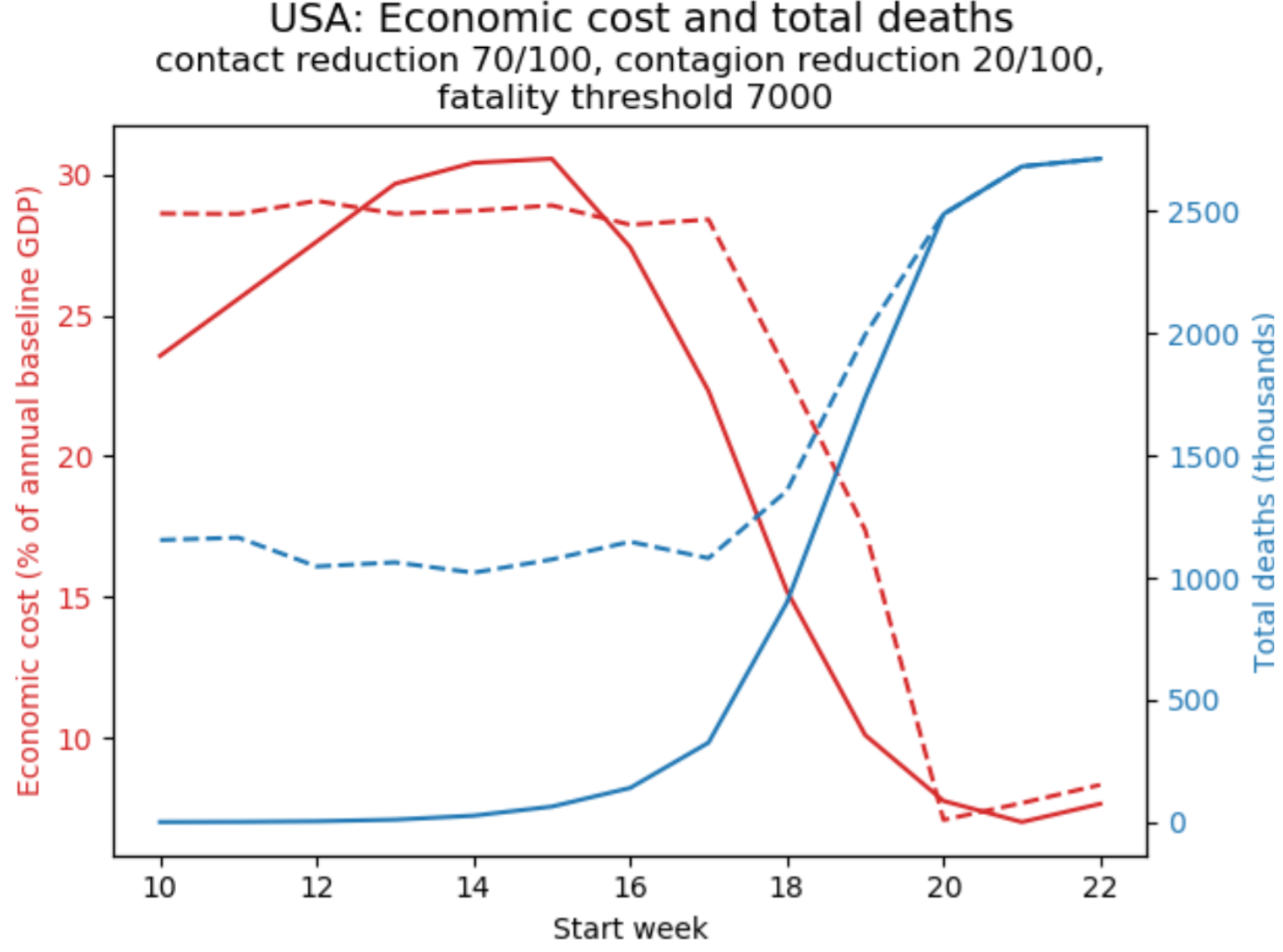
How to read the graphs: Solid curves describe the outcomes of the suppression policy, dashed curves the control policy; economic cost in red (left axis), total fatalities in blue (right axis).
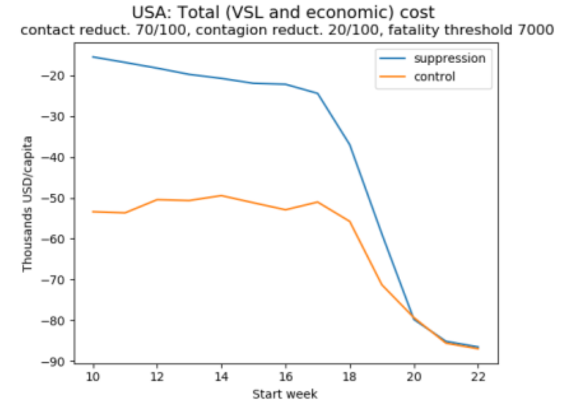
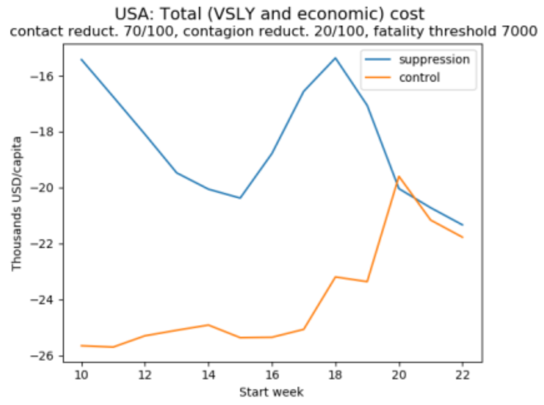
To illustrate how benefit-cost analysis resolves these trade-offs, let’s look at the contrast between an assessment of these projections based on the value of a statistical life (VSL) and one based on statistical life-years (VSLY). This is shown in Figure 2, which displays simulations of the total cost (the sum of the monetary value of lives lost to the crisis and the economic cost) as a function of when the policy is initiated.
Figure 2: Cost-benefit analysis
(a)
(b)
(c)
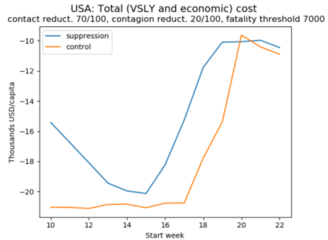
How to read the graphs: The vertical axis displays losses as negative numbers so that the higher on the axis, the better.
Figures 2a-b reveals that both methods favour suppression over control, since the total cost is minimised by the former. Figure 2a also reveals that if we focus on lives saved, then early suppression is clearly superior. By contrast, if we focus on life-years saved, as in Figure 2b, it is acceptable to let the virus spread somewhat before suppression (because in the USA, most victims are elderly and lose relatively few years of life). These two graphs rely on a value of a statistical life equal to 150 times the GDP per capita and a corresponding value of a statistical life year equal to 3 times the GDP per capita. But we noted before that these figures are disputed, and to illustrate how sensitive results are to this assumption, Figure 2c uses a lower value of a statistical life-year equal to one times GDP per capita (roughly what the UK government uses to decide which treatments to include in the NHS) – with the implication that, despite the staggering death toll, delaying policy adoption is reasonable and that very late adoption of either policy is optimal. This underlines the sensitivity of policy assessment in benefit-cost analysis to the value of life (or life year) adopted.
To facilitate comparison with a social welfare analysis of the same projections, we have chosen a measure of wellbeing which aligns with the one implied by benefit-cost analysis. Consequently, in the absence of priority for the worse off, social wellbeing analysis delivers a similar verdict as benefit-cost analysis. But when a degree of priority for the worse-off is introduced, they can differ markedly. In particular, because death results in considerable loss of wellbeing, social welfare analysis tends to give greater weight to health outcomes, something that is further accentuated when fatality rates are higher amongst those who are poor. Likewise, the verdict that social welfare analysis delivers on policies and when they should be initiated will be sensitive to how the economic burdens of their implementation are distributed.
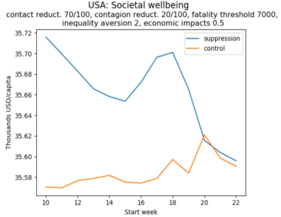
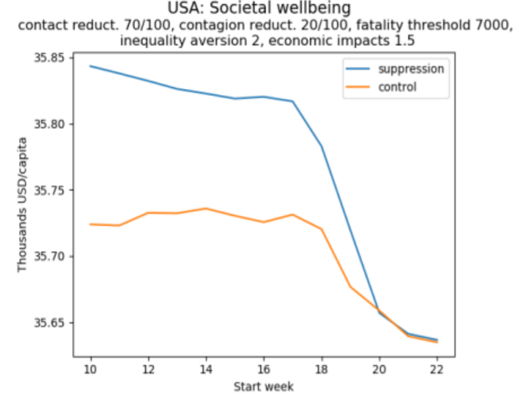
This is illustrated in Figure 3, which uses a measure of societal wellbeing that values a situation by the per capita income which, when equally distributed and associated with equal longevity for everyone, would yield the same overall wellbeing as that situation. Priority for the worse-off (also called “inequality aversion”) is set such that if one individual is half as well-off as another individual, then it is four times more important to give a fixed, small increment in wellbeing to the less well-off person.
Figure 3: The social welfare approach with priority to the worse off
(a)
(b)
How to read these graphs: The vertical axis measures per capita equivalent income. As in Figure 2, the higher the better.
Figure 3a illustrates a situation in which lower income groups in the population bear a disproportionate economic burden, in the sense that the share of income lost declines as individuals get richer. If this burden is heavy, then late adoption of a suppression policy may be preferable to mid-term adoption. Late adoption of a control policy is preferable to any other time. In contrast, Figure 3b illustrates a situation in which there is a progressive distribution of the economic cost. Here, it is always the case that the earlier a policy is implemented, the better.
Although the current crisis presents a difficult trade-off between lives and livelihoods, it is possible to lay out the main considerations that should guide policy, including the key normative parameters for valuing health and economic outcomes and their distribution. Our modelling shows how the relevant empirical and normative elements of sound policy making can be put together into a rigorous framework. It also shows why the social welfare approach, which takes account of the distribution of all aspects of wellbeing and of background inequality, is superior to the benefit-cost approach. Moreover, although model results can at best provide only rough estimates of policy impacts, for reasonable parameters, it suggests that if redistribution mitigates the economic cost to the poorest, then it is likely that the earlier the virus is suppressed, the better.
By Matthew Adler, Richard Bradley, Maddalena Ferranna, Marc Fleurbaey, James Hammitt and Alex Voorhoeve.
Matthew Adler is Richard A. Horvitz Professor of Law and Professor of Economics, Philosophy and Public Policy at Duke University and Lachmann Research Fellow at LSE. His scholarship is interdisciplinary, drawing from welfare economics, normative ethics, and legal theory.
Richard Bradley is Professor of Philosophy at LSE. Much of his work is on individual decision making under uncertainty and the role of hypothetical reasoning in reaching judgements about what to do. He also works on social value and choice.
Maddalena Ferranna is a Research Associate at the Harvard T.H. Chan School of Public Health. She is mainly interested in issues of intra- and inter-generational equity in relation to environmental and health risks. Her current research focuses on establishing a social welfare approach to assess the value of vaccination.
Marc Fleurbaey is Professor at the Paris School of Economics. He was previously Professor of Economics and Humanistic Studies at Princeton University and Lachmann Research Fellow at the LSE. His areas of research are welfare economics, social choice theory, well-being, public economics, and climate policy.
James Hammitt is Professor of Economics and Decision Sciences in the Departments of Health Policy and Management and of Environmental Health, and Director of the Harvard Center for Risk Analysis. His research focuses on the development and application of quantitative methods to health and environmental policy, including benefit-cost, decision, and risk analysis.
Alex Voorhoeve is Professor of Philosophy at the LSE and part-time Visiting Professor of Ethics and Economics at Erasmus University Rotterdam. He works on the theory and practice of distributive justice (especially as it relates to health), on rational choice theory and moral psychology.